Price Elasticity of Demand: The Formula, the Curves and What the Number Means
A price rise can raise a seller's revenue or cut it, and the difference is how strongly buyers respond. Elasticity is the number that measures that response.
A tax can raise the price without cutting purchases very much
A government deciding whether to tax cigarettes faces two outcomes at once: fewer cigarettes may be consumed, while the higher price may still raise tax receipts. A 2015 systematic review of 32 studies in Latin America and the Caribbean estimated cigarette-demand price elasticity at −0.31 in the short run and −0.43 in the long run. In that review, a 10% price increase therefore corresponds, approximately, to a 3.1% short-run and 4.3% long-run fall in consumption—not a 10% fall [1]. The estimates are averages across studies, not a forecast for every country or tax design.
That is the decision problem elasticity helps solve. A small response in quantity lets a seller keep much of its volume after a price rise, and lets a tax change behaviour more slowly than policymakers hope. The burden does not stay with the seller: who pays depends on how prices, wages, profits and alternatives adjust across the market.
The measure matters beyond tobacco. A 2012 meta-analysis of gasoline-demand studies found a corrected average elasticity of −0.09 in the short run and −0.31 in the long run [2]. Drivers cannot immediately change their cars, homes or commute; over time they can buy a more efficient vehicle, move or change transport modes. A price response is a property of a market over a specified horizon, not a permanent label attached to a product.
The formula, and the sign trap
Price elasticity of demand measures the percentage change in quantity demanded divided by the percentage change in price:
E = (percentage change in quantity demanded) ÷ (percentage change in price)
For an ordinary downward-sloping demand curve, price and quantity move in opposite directions, so the coefficient is negative. If price rises by 1% and quantity falls by 1.4%, then E = −1.4. Many textbooks compare the absolute value, |E| = 1.4, so that "more elastic" means a larger response without the minus sign. The sign still describes the direction of the relationship.
There are two common ways to calculate it. The point method measures percentage changes from a chosen base, or the local slope where a demand function is known, and can give a different answer depending on which endpoint is the base. The midpoint, or arc, method avoids that asymmetry by dividing each change by the average of the two endpoints:
E = [(Q₂ − Q₁) ÷ ((Q₁ + Q₂) ÷ 2)] ÷ [(P₂ − P₁) ÷ ((P₁ + P₂) ÷ 2)]
Use the midpoint method to compare two observed price–quantity pairs; use point elasticity for a small change around a known point. Both are local or interval measures, and neither promises the same response after a much larger price change.
A worked calculation, from two observations to one coefficient
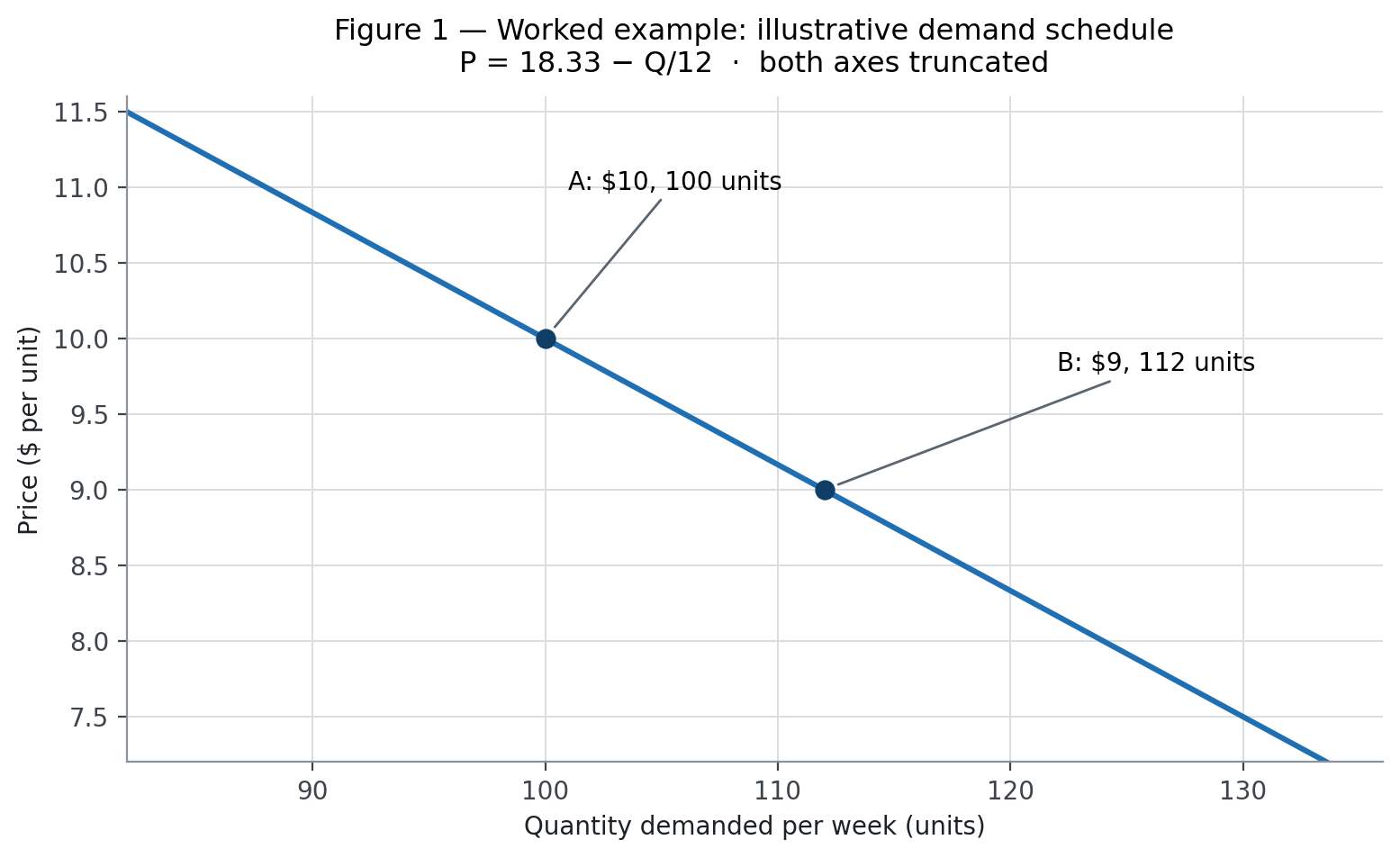
Suppose a shop sells 100 units a week at $10 each. After the price falls to $9, weekly sales rise to 112 units. These are hypothetical teaching figures, not observations from a real company.
Using the midpoint method:
- Quantity change: 112 − 100 = 12 units. Average quantity: (112 + 100) ÷ 2 = 106. Percentage change: 12 ÷ 106 = 11.32%.
- Price change: 9 − 10 = −1. Average price: (9 + 10) ÷ 2 = 9.50. Percentage change: −1 ÷ 9.50 = −10.53%.
- Divide the quantity change by the price change: 11.32% ÷ −10.53% = −1.08.
The estimated arc elasticity is −1.08; its absolute value is 1.08, just above one. Over this interval, quantity demanded changed slightly more, in percentage terms, than price. In plain terms, a 1% price rise would cut quantity by about 1.08% if the same elasticity applied locally — an interval estimate, not a law for every price.
The five cases: read the curve and the coefficient together
Economics classes distinguish five benchmark cases. Elasticity is not simply the steepness of a line: the coefficient also depends on the price and quantity at the point measured. The five panels below use constant-elasticity curves—|E| = 2, 0.5 and 1—so each label holds along the whole curve; a straight line instead runs from elastic at high prices to inelastic at low ones, unit elastic only at its midpoint.
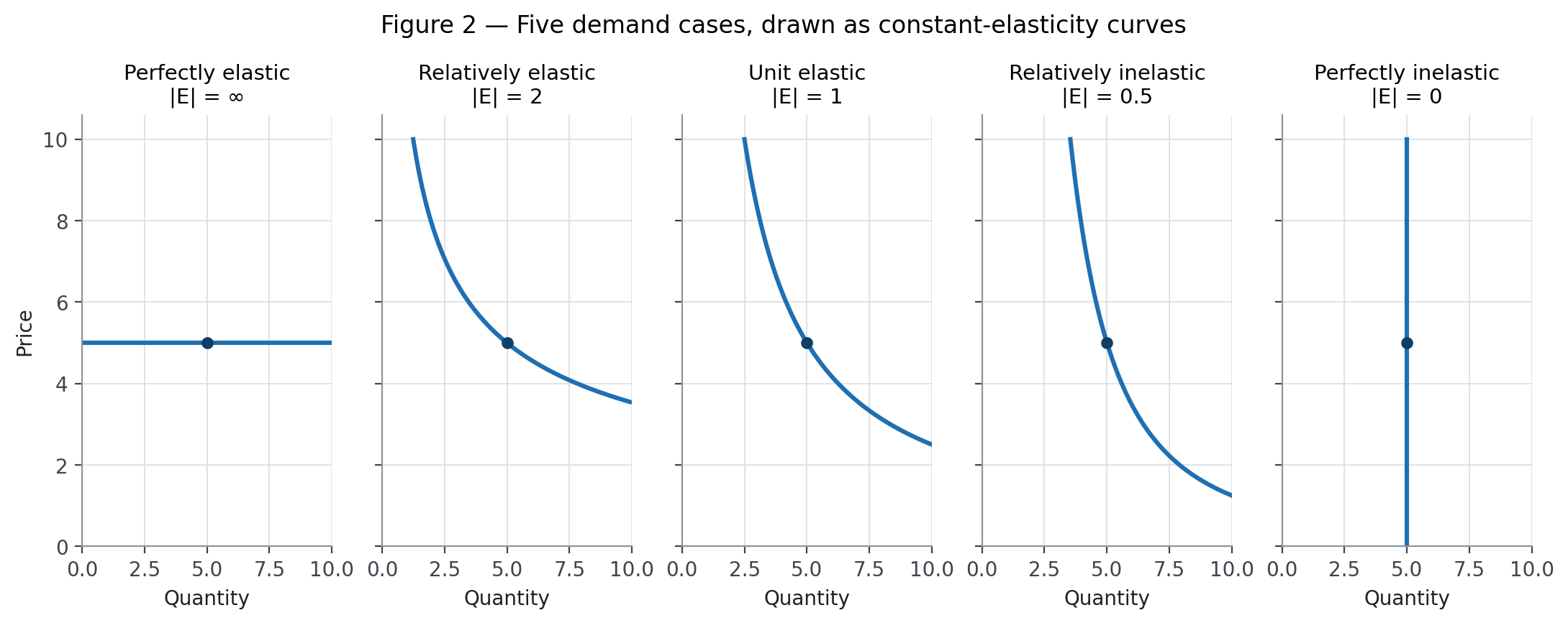
- Perfectly elastic — |E| = ∞. The curve is horizontal: buyers will purchase at the market price, but demand from the individual seller disappears if it charges more. A competitive seller facing a market price is the textbook approximation; no real market is perfectly elastic in every circumstance.
- Relatively elastic — |E| > 1. Quantity changes by a greater percentage than price. A differentiated product with close alternatives can approach this case. Even responsive categories often stay just below one: the 2010 review of US food-demand studies found absolute mean elasticities of 0.79 for soft drinks and 0.81 for food away from home [3].
- Unit elastic — |E| = 1. Percentage changes in price and quantity are equal in magnitude. On a straight-line demand curve, this occurs at its midpoint; on a constant-elasticity curve, it holds throughout. It is a useful benchmark, not a claim that every observed market contains a precisely unit-elastic point.
- Relatively inelastic — 0 < |E| < 1. Quantity changes by a smaller percentage than price. Electricity demand is an example of a market that is often inelastic in the short run: a 2025 meta-analysis of 4,521 estimates from 413 studies reported average short-run elasticity of −0.231 and long-run elasticity of −0.532 before its publication-bias correction [4]. Those estimates become smaller in magnitude after correction.
- Perfectly inelastic — |E| = 0. The curve is vertical: quantity does not respond to price. This is a limiting model, sometimes used to explain a fixed short-run requirement, not a literal description of all purchases of a real product.
For the broader taxonomy, see the site's pages on types of elasticity and types of elasticity of demand; cross elasticity of demand covers the response to another good's price, and income elasticity the response to income.
Elastic versus inelastic: a side-by-side test
The two categories differ on five counts, and the revenue row is the one that changes decisions.
- Absolute coefficient. Elastic demand is above 1; inelastic demand sits between 0 and 1.
- Quantity response. Elastic: a larger percentage change than the price change. Inelastic: a smaller one.
- Shape of the curve, with price on the vertical axis: relatively flatter around the point when elastic, relatively steeper when inelastic. On a straight line, the flatness is not the whole story—the same curve is elastic at high prices and inelastic at low ones.
- Revenue when price rises. It tends to fall when demand is elastic and to rise when demand is inelastic.
- Typical examples, as rules of thumb rather than laws: leisure travel and branded goods with close substitutes on the elastic side; short-run electricity use and cigarettes in many studies on the inelastic side.
The verbal test: if price changes by 1%, does quantity change by more than 1% in the opposite direction? If yes, demand is elastic; less than 1%, inelastic; exactly 1%, unit elastic. These labels apply to a point or interval, and a product can move between categories as price, alternatives and horizon change.
What makes demand more or less elastic?
Five mechanisms explain much of the variation.
Substitutes. The more credible alternatives buyers have, the easier it is to leave when price rises. A branded cereal facing several similar brands may lose customers after a price increase; a remote village with one fuel station has fewer immediate alternatives. The relevant substitutes must be available, acceptable and affordable—not merely imaginable.
Budget share. A 10% increase in a cheap condiment barely touches a household budget; the same increase in rent is harder to ignore. A large budget share gives buyers a stronger incentive to search, postpone or cut.
Necessity versus luxury. Households have fewer options to cut essential electricity use immediately than to postpone a nonessential restaurant meal. The 2025 electricity meta-analysis found a corrected short-run average of −0.116 and long-run average of −0.303, showing both inelasticity and a larger response over time [4]. The classification is relative: necessities become more responsive as substitutes or efficiency investments appear.
Time horizon. In the short run, a commuter may keep buying fuel because work, vehicle and housing choices are fixed. Over years, that person may move closer to work or switch vehicles. The gasoline meta-analysis' corrected averages—−0.09 short run and −0.31 long run, published in 2012—illustrate the mechanism [2]. They are cross-study averages, not current forecasts for a particular country.
Complements. Goods used together affect one another's demand. If running a petrol car becomes more expensive, demand for fuel-efficient cars or public transport may rise. This is cross-price elasticity, not own-price elasticity: the sign depends on whether the other good is a substitute or a complement.
The total-revenue test: why the same price rise can help or hurt
Total revenue is price times quantity: TR = P × Q. In the schedule from Figure 1, $10 and 100 units give $1,000; $9 and 112 units give $1,008. The price cut adds $8 because the quantity response more than offsets the lower price over this illustrative interval — arithmetic, not evidence about a real shop.
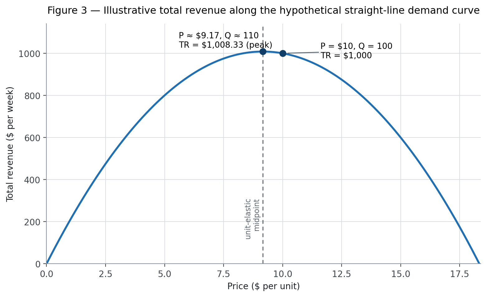
The rule for a small price change is: on an elastic stretch, a price rise reduces total revenue because the percentage fall in quantity is larger than the percentage rise in price. On an inelastic stretch, a price rise increases revenue because quantity falls proportionally less. At unit elasticity, revenue is locally unchanged; for a linear demand curve it peaks at the midpoint, which here is $1,008.33. This is a revenue rule, not a profit rule: profit also depends on costs, capacity and how customers respond to discounts.
What published estimates say, and why they disagree
Estimates are not constants engraved on a product: they vary with the period, country, population, aggregation, treatment of substitutes and method. The figure compares published averages and category means without pretending they are interchangeable.
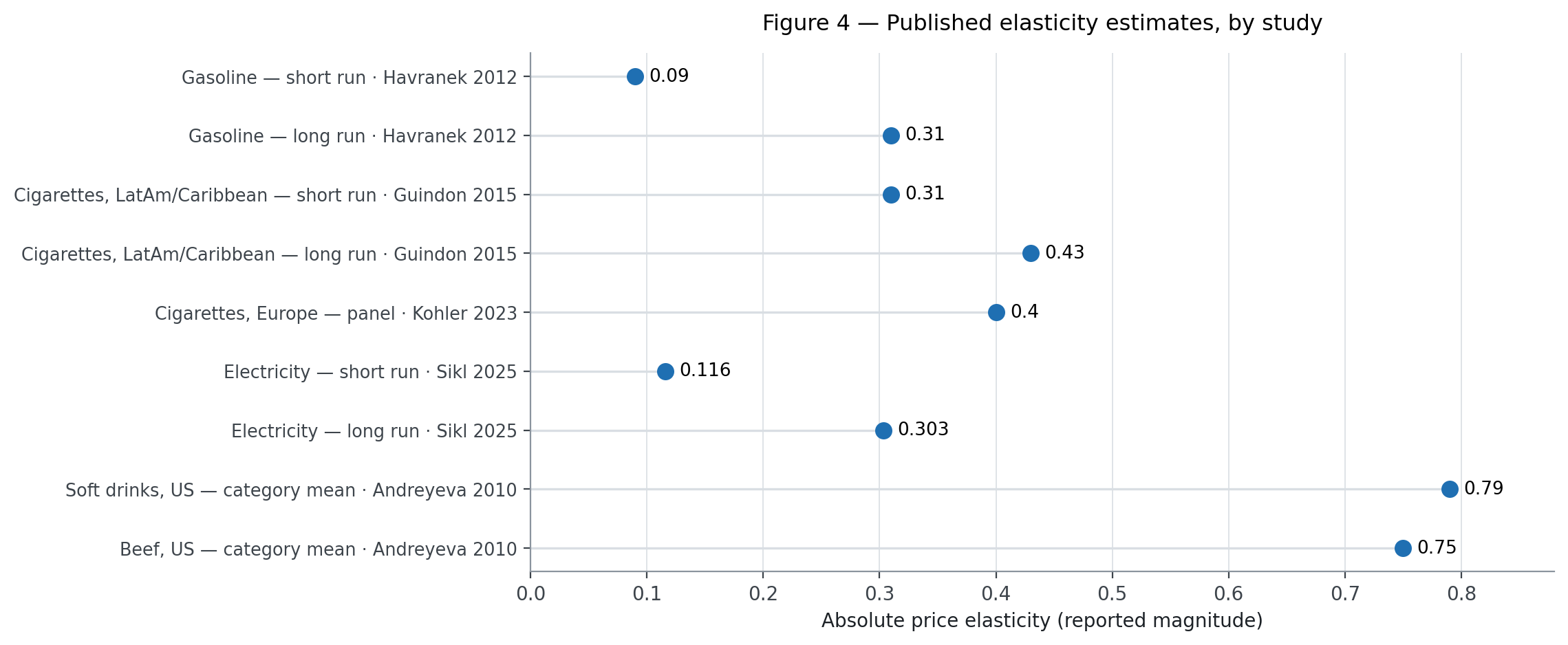
The ranges can be material even within one product category. The 2015 Latin America and Caribbean cigarette review pooled short-run elasticity at −0.31 (95% confidence interval −0.39 to −0.24) and long-run elasticity at −0.43 (−0.51 to −0.35), but individual country studies varied. Studies from Argentina, Chile and Mexico in that review clustered in narrow ranges: −0.10 to −0.30 in the short run and −0.25 to −0.45 in the long run [1]. A 2023 European cigarette study by Kohler, Vinci and Mattli estimated around −0.4 from panel data for 2010–2020, with a 95% confidence interval of −0.67 to −0.24 [5]. Different samples and models answer related, not identical, questions.
The electricity literature shows why method matters. The 2025 meta-analysis reported raw averages of −0.231 short run and −0.532 long run across 4,521 estimates from 413 studies; after correcting for publication bias, the averages fell to −0.116 and −0.303 [4]. In food, a 2010 systematic review of 160 studies reported US mean absolute elasticities from 0.27 for eggs to 0.79 for soft drinks and 0.75 for beef, using estimates covering 1938–2007 [3]. The review's category averages conceal wide ranges: the individual soft-drink estimates it collected ran from 0.13 to 3.18.
The message is not that elasticity is useless because estimates disagree. It is that an estimate must travel with its market, period, horizon and method. The chart's nine observations are benchmarks from published reviews, not a harmonised experiment. Before using a coefficient for a forecast, ask whether the population, substitutes and time horizon resemble the decision at hand.
Why it matters for households, firms and governments
Tax incidence. A tax creates a wedge between what buyers pay and sellers receive. The side of the market that is less responsive to price generally bears more of the economic burden, regardless of which side legally remits the tax. With inelastic cigarette demand, taxes can raise substantial revenue while reducing consumption less than proportionally; the actual result also depends on pass-through, illicit supply, product switching and the policy objective. The 2015 regional review found that higher cigarette prices reduced consumption, but also noted the shortage of household- and individual-level evidence in the region [1].
Price controls. A legal price ceiling below the market-clearing level can increase quantity demanded while discouraging supply. Elasticity helps quantify the demand response, but shortages also depend on supply elasticity, rationing rules, quality changes and enforcement.
Discounts and business decisions. A firm should not assume that a lower price means higher revenue. It should estimate the incremental quantity sold, include the effect on full-price sales and compare contribution margins. Even a revenue-raising discount can reduce profit if the extra units do not cover variable costs or if customers merely bring purchases forward.
Why governments tax inelastic goods. Inelastic demand can make a tax a reliable revenue source because quantity contracts relatively little. But a stable tax base is not a good policy by itself: tobacco taxes also aim to cut harmful consumption, while taxes on essentials can weigh on low-income households. The evaluation combines demand response with health effects, distribution and how revenue is used.
Elasticity is best treated as a decision tool with a defined scope. The formula makes responses comparable; the estimate's context determines whether it is useful. A coefficient without a market, period and method is a number without enough meaning.
Sources and further reading
- Guindon, Paraje and Chaloupka, "The Impact of Prices and Taxes on the Use of Tobacco Products in Latin America and the Caribbean" (2015). Systematic review of 32 studies; pooled cigarette-demand elasticities and country variation.
- Havranek, Irsova and Janda, "Demand for gasoline is more price-inelastic than commonly thought" (2012). Meta-analysis and publication-bias-corrected short- and long-run gasoline elasticities.
- Andreyeva, Long and Brownell, "The Impact of Food Prices on Consumption: A Systematic Review of Research on the Price Elasticity of Demand for Food" (2010). Review of 160 studies; US food and beverage category estimates covering 1938–2007.
- Sikl, Irsova, Kudela and Kudelova, "Price Elasticity of Electricity Revisited: A Meta-Analysis" (2025). Meta-analysis of 4,521 estimates from 413 studies; raw and publication-bias-corrected electricity elasticities.
- Kohler, Vinci and Mattli, "Cross-country and panel data estimates of the price elasticity of demand for cigarettes in Europe" (2023). European cigarette-demand estimates using data from 2010–2020 and panel methods.
See also: Demand in Economics, Demand Function, Types of Elasticity of Demand, Cross Elasticity of Demand.