Indifference curves: the trade-offs behind consumer demand
An indifference curve is the set of bundles of two goods that a consumer ranks equally. Combined with a budget line it narrows what that consumer can choose, and it is the model behind the demand curve.
What an indifference curve is
Put the quantity of one good on the horizontal axis and the quantity of another on the vertical axis. Every point is a consumption bundle: 3 units of A and 7 of B, for example. An indifference curve joins the bundles the consumer ranks equally. Moving along it changes what is consumed, but not the consumer's ranking of the bundle.
Utility in this model is ordinal. It can say that one bundle ranks above, below or level with another; it does not say that one gives 20% more satisfaction. The labels sometimes attached to curves are therefore names, not measurements. Any relabeling that preserves their order describes the same preferences.[1]
That distinction matters because the familiar downward-sloping, bowed-in curve is an assumption about preferences. It is not a shape discovered in a survey, nor evidence that people carry a utility function in their heads. The drawing assumes that more of either good is preferred to less and that balanced mixtures are preferred to extremes. Change those assumptions and the shape changes.[1]
The marginal rate of substitution
The slope of a curve is the marginal rate of substitution, or MRS: the amount of B the consumer would give up for one more unit of A while remaining equally well off. Economists often report its absolute value so that a trade-off of 6 units of B for 1 of A is written as an MRS of 6 rather than a slope of -6.[1]
The ordinary curve is convex toward the origin. On the left of Figure 1, A is scarce and B is plentiful, so the consumer is willing to surrender 6 units of B for another unit of A. Farther right, A is plentiful and B is scarce, and that willingness falls to 0.375. This is diminishing MRS. Convexity is the preference assumption that averages are at least as good as extremes; strict convexity makes the average strictly better.[1]
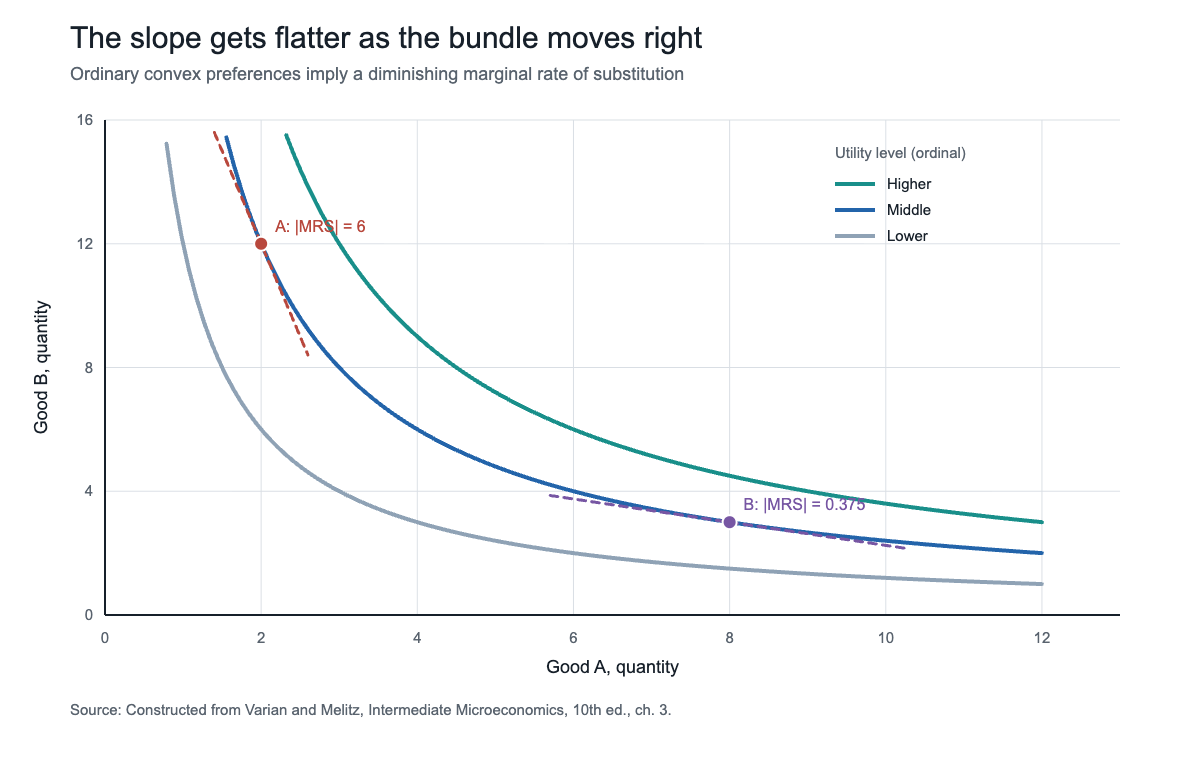
A flatter curve does not mean the consumer cares less in any absolute sense. It means the local exchange rate between the two goods has changed. The curve is a map of willingness to trade, bundle by bundle.
Indifference curves and the budget line
Preferences say what the consumer wants; the budget line says what is possible. If income is m and prices are pA and pB, affordable bundles satisfy pA x A + pB x B <= m. The boundary has slope -pA/pB: the market requires the consumer to give up pA/pB units of B to obtain one more unit of A.[1]
For an interior choice with smooth, convex preferences, the highest attainable indifference curve is tangent to that line. The familiar condition MRS = pA/pB is plain language dressed as algebra: the rate at which the consumer is willing to trade equals the rate at which the market permits the trade. If those rates differ, moving along the budget line can reach a preferred bundle. A tangency is a model solution, not a claim that shoppers calculate derivatives.[1]
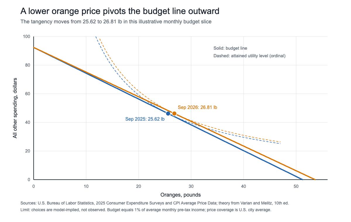
Figure 2 gives the geometry real scale. The U.S. Bureau of Labor Statistics reported average pre-tax income of $110,847 per consumer unit in 2025, or $9,237.25 a month, in a release dated October 29, 2026.[2] The figure sets aside 1% of that monthly amount, $92.37, for oranges and an all-other-spending composite. BLS's U.S. city average price for navel oranges fell from $1.803 a pound in September 2025 to $1.723 in September 2026, a 4.4% decline.[3]
With the illustrative Cobb-Douglas preference in the caption, half the budget goes to each side. The price change pivots the line outward and shifts the modeled tangency from 25.62 pounds to 26.81 pounds. Those quantities are not observed purchases. They isolate the mechanism: a lower relative price expands the affordable set and changes the bundle that best fits the assumed preferences.
Indifference curves for perfect substitutes and perfect complements
Perfect substitutes have straight, parallel indifference curves. For one-for-one substitutes represented by U = A + B, the MRS is always 1. If A costs less than B, every dollar buys more utility through A, so the optimum is the corner with only A. If prices are equal, every affordable mix on the budget line ranks equally. More generally, the consumer compares price per unit of the service each good provides, not merely the sticker prices.[1]
Perfect complements have L-shaped curves. With U = min(A, B), an extra unit of A adds nothing unless B also rises, so useful consumption occurs in a fixed 1:1 proportion. The optimum is normally at the kink. The MRS is not a smooth trade-off there: along one arm it is zero and along the other it is effectively infinite. A price change can alter how many pairs the consumer can afford, but it does not induce substitution between the components.[1]
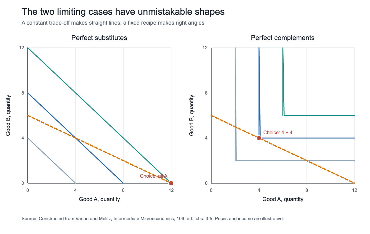
Most goods are imperfect substitutes. Tea may replace some coffee, but not cup for cup for every consumer and at every quantity. The ordinary convex curve is the workhorse because it permits substitution while making the willingness to substitute depend on the starting bundle. It sits between the constant trade-off of a straight line and the zero-at-the-margin substitution of a right angle. Calling it ordinary is a modeling convention, not a statistical claim that every real preference has that shape.
From indifference curves to the demand curve
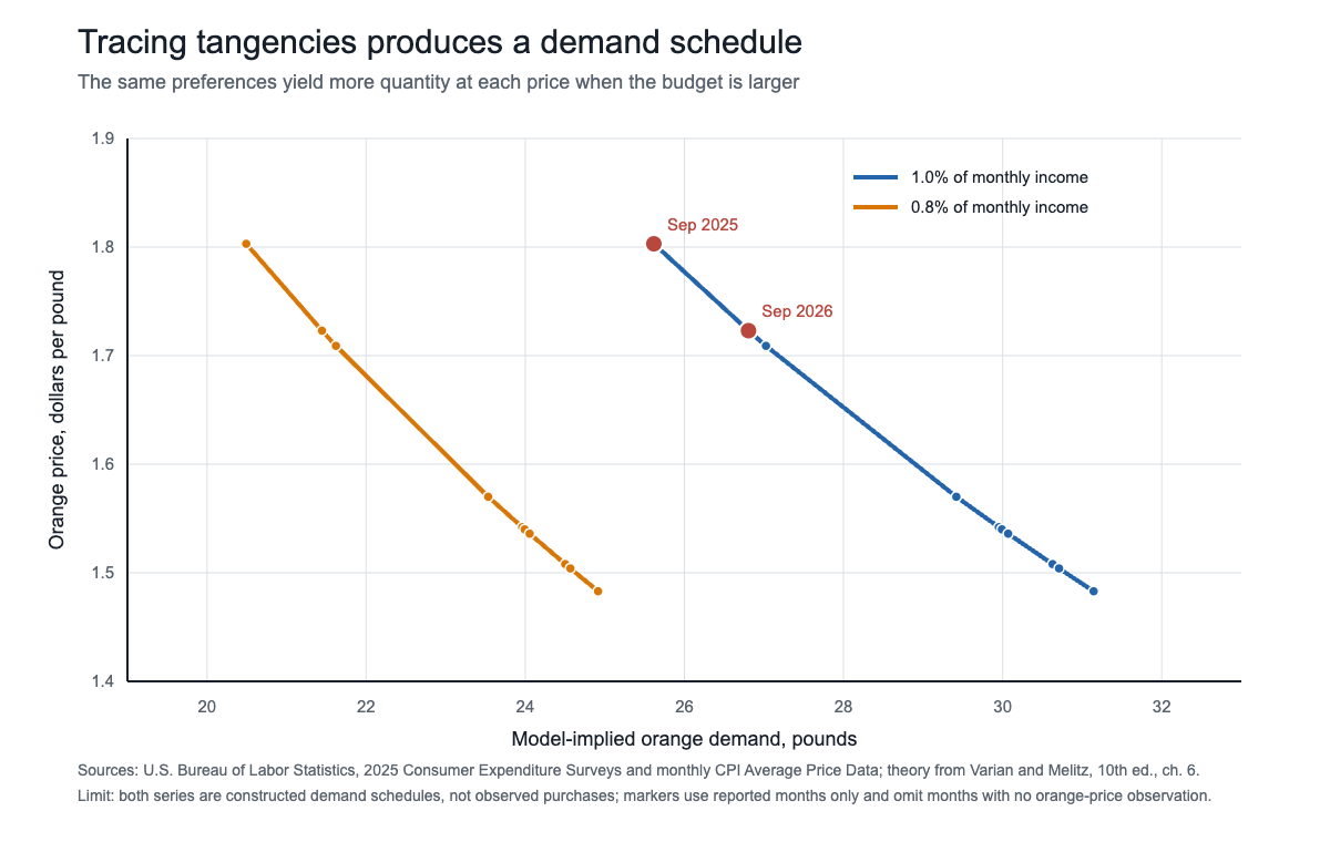
Hold income, the other price and preferences fixed. Change the price of A, pivot the budget line and record the chosen quantity of A at each new tangency. Plot those price-quantity pairs in a separate panel and the individual demand curve appears. In the Cobb-Douglas example used here, orange demand is q = m/(2p), so quantity falls as price rises.[1]
Figure 4 applies that equation to reported BLS orange prices for 10 months from September 2025 through September 2026. Months without a reported navel-orange price are omitted rather than interpolated.[3] At every reported price, the schedule based on 1% of average monthly income lies to the right of the schedule based on 0.8%. That is the income channel: a larger affordable set supports a larger quantity at the same price. The marked September points are the two tangencies in Figure 2.
The same logic scales from a household to a market. Add quantities across consumers at each price and the individual schedules become market demand. That link is why assumptions about substitution matter for taxes, inflation and policy: they determine how much a price change reduces quantity, how much spending shifts toward alternatives and how strongly a loss of purchasing power reaches other markets.[1]
The limits of the model
The curves on this page are not estimates of utility. In revealed-preference analysis, observed choices instead impose consistency restrictions. If a consumer chooses bundle A when B was affordable, A is revealed to rank at least as high as B. Across repeated budget situations, those choices must not form a cycle that contradicts a stable ranking. Modern revealed-preference work uses those restrictions to bound and predict demand without claiming to observe satisfaction directly.[4]
That is narrower than a psychological theory. The model leaves out advertising, habits, mistaken forecasts, changing attention and social context unless they are built into the choice problem. A review in the Journal of Economic Literature documented systematic preference reversals and concluded that choices can depend on the environment in which preferences are elicited.[5] Such evidence does not make budget constraints disappear; it warns against treating one fixed map of curves as a literal portrait of the mind.
The extremes are most credible when the technology of consumption enforces them. A left shoe and a right shoe are close to perfect 1:1 complements for wearing a pair.[1] Gasoline and driving are not. In December 2014, the U.S. Energy Information Administration put the short-run price elasticity of U.S. motor-gasoline demand between -0.02 and -0.04: small, but not zero. Over time, drivers can alter trips, vehicles and fuel economy, so an L-shape that predicts no substitution misses available adjustments.[6]
The safe reading is therefore conditional: if rankings are stable, if the two-good description captures the relevant alternatives, and if the assumed curve shape is reasonable, then prices and income predict a choice. The value of the diagram is that it makes each condition visible. Its danger is forgetting that the smooth curve came from the analyst, not from a utility meter.
Sources and further reading
- W. W. Norton, Intermediate Microeconomics: A Modern Approach, 10th ed., by Hal R. Varian and Marc J. Melitz (2024). Chapters 2-7 support budget constraints, preferences, utility, choice, demand and revealed preference.
- U.S. Bureau of Labor Statistics, "Consumer Expenditures--2025" (29 October 2026). Supports average 2025 pre-tax income and the survey's consumer-unit definition.
- U.S. Bureau of Labor Statistics, "Average price data (in U.S. dollars), selected items" (September 2026 release). Supports monthly U.S. city average navel-orange prices.
- American Economic Association, "Mutually Consistent Revealed Preference Demand Predictions" by Abi Adams (February 2020). Supports the use of revealed-preference restrictions to make rational demand predictions across budgets.
- American Economic Association, "Extending the Bounds of Rationality: Evidence and Theories of Preferential Choice" by Jörg Rieskamp, Jerome R. Busemeyer and Barbara A. Mellers (September 2006). Supports the evidence on preference reversals and context-dependent choice.
- U.S. Energy Information Administration, "Gasoline prices tend to have little effect on demand for car travel" (15 December 2014). Supports the cited short-run gasoline price-elasticity range and the mechanisms that prevent zero substitution.
See also: Perfect Substitute Goods, Substitute Goods, Price Elasticity of Demand: The Formula, the Curves and What the Number Means.