Supply in economics: the supply curve and what shifts it

By: EconomicPoint

Supply is the quantity of a good or service producers are willing and able to offer at each price over a stated period.

What supply means

Supply describes a producer's selling plans under specified conditions. A quantity supplied is the amount offered at one particular price. The supply curve collects those price and quantity combinations while holding other influences constant, including input prices, technology and the period available for adjustment. [1]

Consider a hypothetical baker with capacity for 100 loaves a day. At a posted price of US$4 a loaf, the baker plans to offer 40, but customers buy only 30. Capacity is 100, quantity supplied is 40, and sales are 30. Counting the loaves in the shop would establish an inventory at a moment in time. It would not reveal how many the baker would offer tomorrow at a different price.

The period and product must stay consistent. Forty loaves per day cannot be compared directly with 40 per week, and a price for an ordinary loaf cannot be paired with the quantity of all baked goods. The competitive model also assumes that each seller takes the market price as given. It holds the pursuit of profit constant and explains the upward slope through the cost of producing additional units. [1]

The supply schedule and the supply curve

A supply schedule lists the quantities offered at alternative prices. The following constructed example describes two bakers selling identical loaves in the same market. Each row refers to a possible price for the same illustrative day, with other conditions unchanged. It does not record three successive days. The numerical schedules are chosen for teaching; the definitions follow the 2022 textbook. [1]

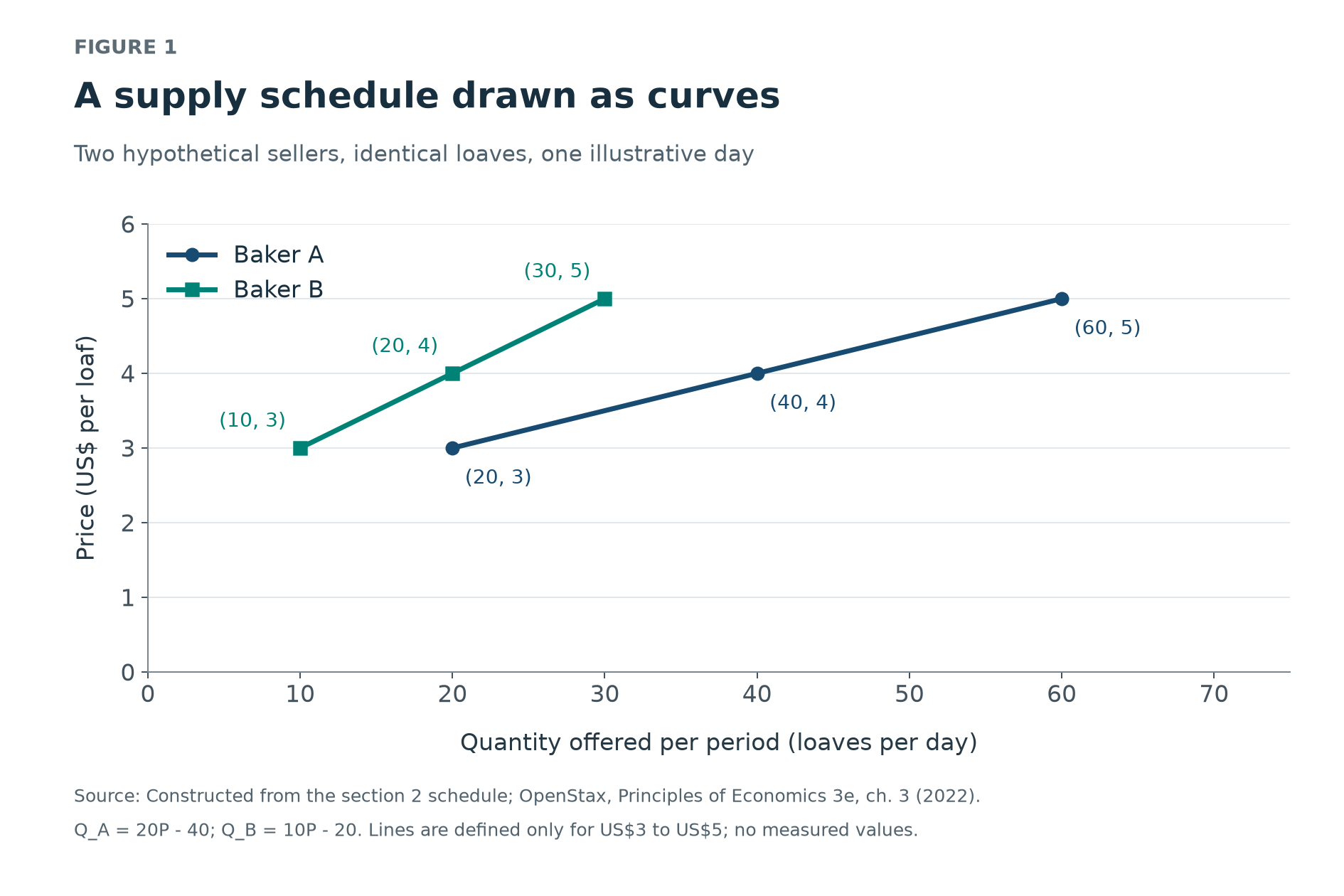
| Price per loaf | Baker A: loaves offered per day | Baker B: loaves offered per day | |---|---:|---:| | US$3 | 20 | 10 | | US$4 | 40 | 20 | | US$5 | 60 | 30 |

Price goes on the vertical axis and quantity offered per period on the horizontal axis. To plot baker A's middle row, start at 40 loaves horizontally and US$4 vertically. Repeating this for the other rows draws A's supply curve. A straight supply line is one possible shape; the word "curve" also covers a straight line. [1]

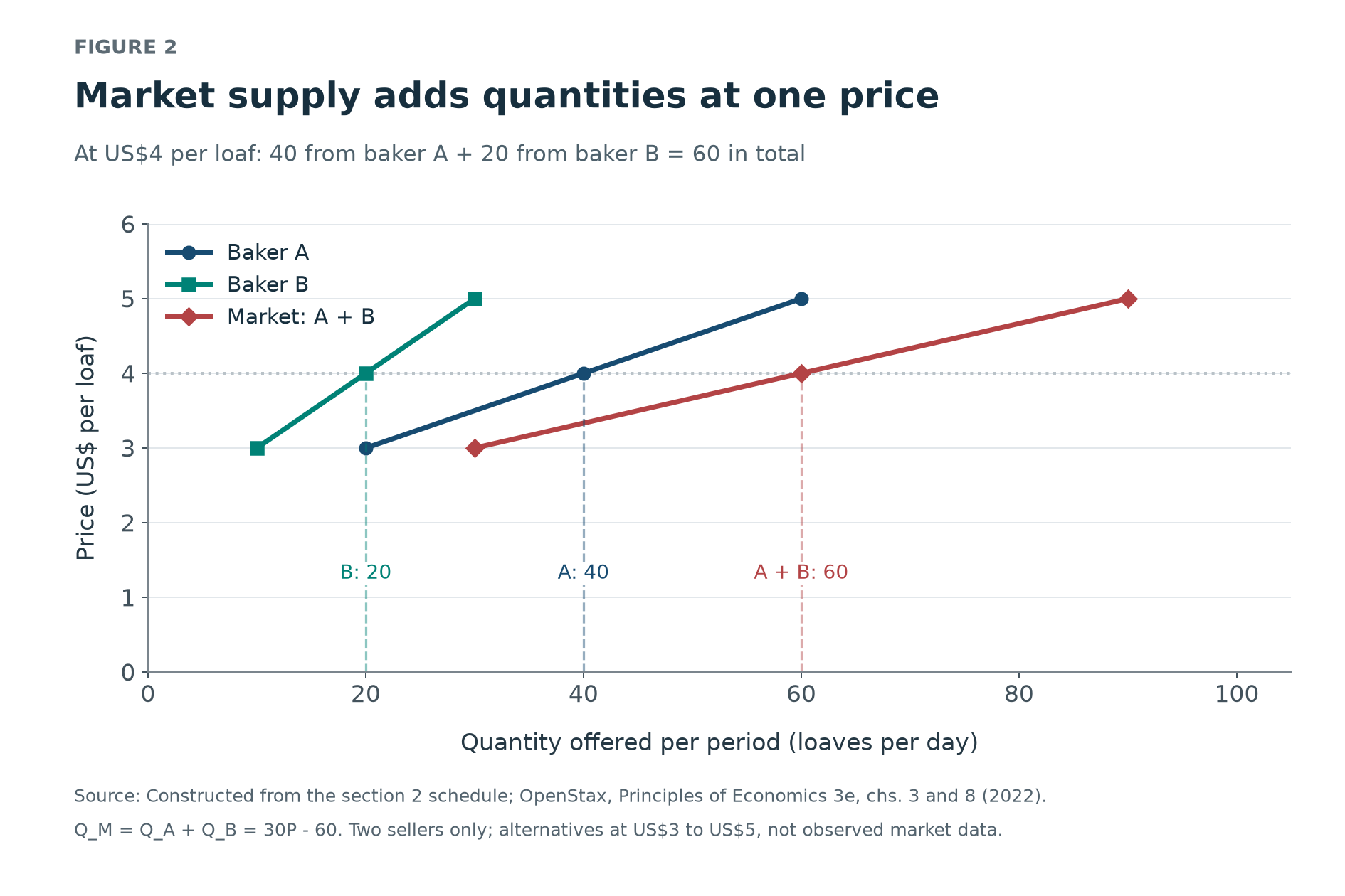
Figure 1. Two supply schedules drawn as curves. Constructed from the schedule in section 2, with Q_A = 20P - 40 and Q_B = 10P - 20, where P is US$ per loaf and Q is loaves per day. Lines show these stated linear forms only between US$3 and US$5. These are hypothetical alternatives for one day, not observations. Definition source: OpenStax, Principles of Economics, third edition, chapter 3, section 3.1 (2022).

Market supply adds the sellers' quantities at a common price. At US$3, the total is 20 + 10 = 30 loaves. At US$4, it is 40 + 20 = 60. At US$5, it is 60 + 30 = 90. This gives a market schedule of 30, 60 and 90 loaves per day. The horizontal distances add because both sellers face the same price. [1][5]

Figure 2. Individual supply and their horizontal sum. Constructed from the section 2 schedules: Q_A = 20P - 40, Q_B = 10P - 20 and Q_M = 30P - 60, for prices from US$3 to US$5. At US$4, 40 plus 20 equals 60 loaves offered per day. Only these two hypothetical sellers are included; this is not an estimated market curve. Definition source: OpenStax, Principles of Economics, third edition, chapter 3, section 3.1 and chapter 8, section 8.2 (2022).

Movement along the supply curve and shifts in supply

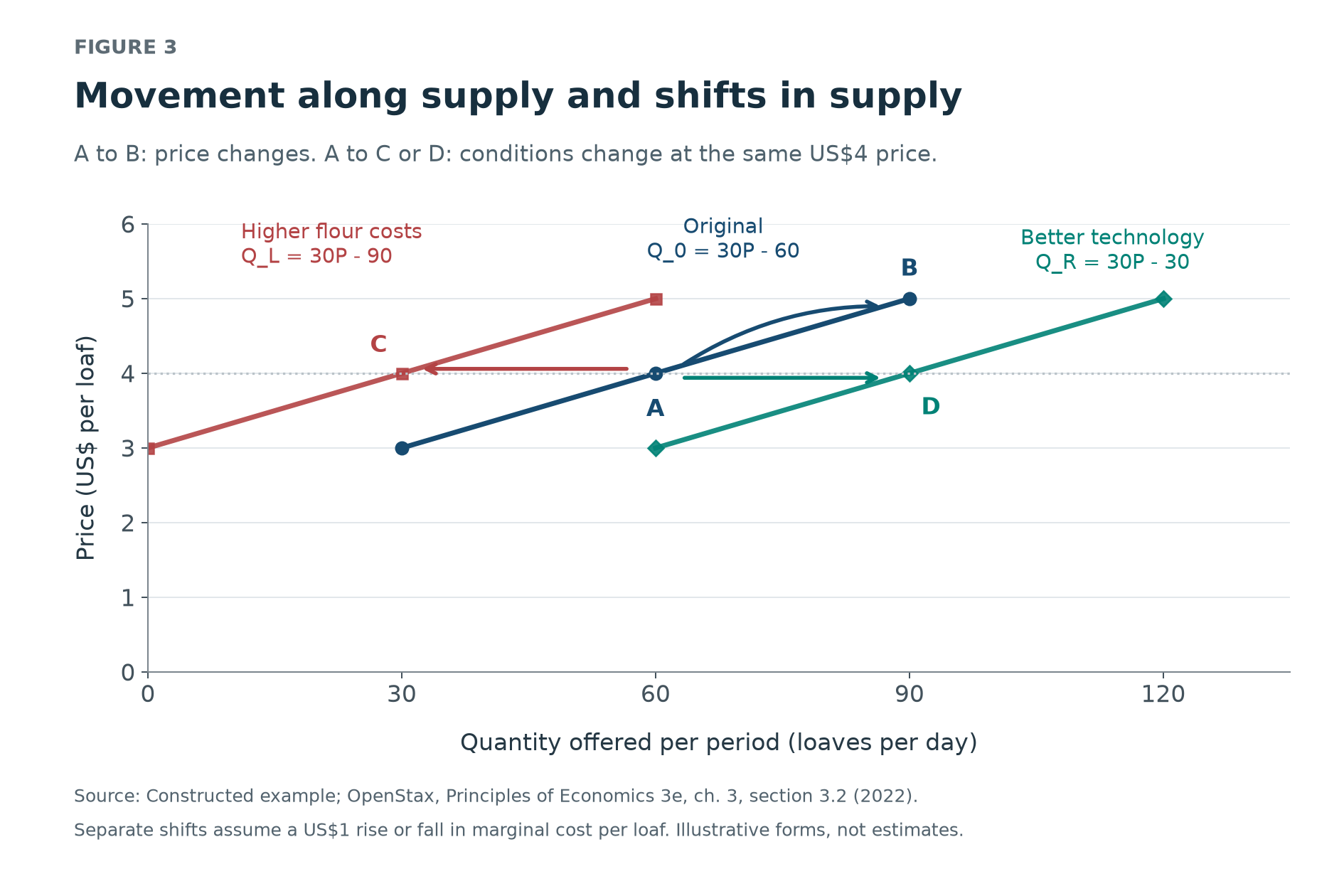
A change in the product's own price changes quantity supplied along the existing curve. In the constructed market, a rise from US$4 to US$5 increases quantity supplied from 60 to 90 loaves per day. The selling conditions represented by the curve remain fixed. The change is a movement from A to B in Figure 3. [2]

A shift changes the quantity offered at a given price. Suppose more expensive flour adds US$1 to the marginal cost of each loaf for both bakers. In this example, a US$4 selling price then induces the quantity previously offered at US$3: 30 loaves altogether. The supply curve shifts left. Alternatively, suppose an improved production method saves US$1 per additional loaf. At US$4, sellers then offer 90 loaves, shifting supply right. These are separate hypothetical changes from the same starting position. [2]

Figure 3. A price movement compared with two supply shifts. Constructed forms are Q_0 = 30P - 60, Q_L = 30P - 90 and Q_R = 30P - 30, for US$3 to US$5 per loaf. A to B is movement along Q_0. At the unchanged US$4 price, higher flour costs reduce quantity from 60 to 30, while a separate technology improvement raises it to 90. The assumed cost changes are illustrative, not measured. Definition source: OpenStax, Principles of Economics, third edition, chapter 3, section 3.2 (2022).

Input prices and technology are among the conditions held fixed when drawing a curve. A tax per unit sold adds to the cost of supplying that unit and shifts supply left when the vertical axis measures the buyer's price. A subsidy per unit supplied works in the opposite direction. A fixed annual charge need not change an operating firm's marginal cost, although it can affect entry and exit. [2][5][6]

The number of sellers changes market supply through the same addition used above. If another baker identical to B enters, quantity offered at US$4 rises from 60 to 80 loaves per day. Expectations also affect current offers: a seller of a storable commodity expecting a higher future price may withhold stocks today if the expected gain covers storage costs. That can reduce current supply even though today's price has not changed. [3]

Marginal cost and the firm's supply decision

Marginal cost is the extra cost of producing another unit. In the short run, some inputs are fixed. Adding workers to an unchanged oven eventually produces smaller additions to output per worker. With wages unchanged, producing an extra loaf then requires more spending on labor. Marginal cost rises. This diminishing marginal productivity explains the upward-sloping portion of the cost curve; it need not apply at every output level. [4]

For a competitive firm, selling another unit adds the market price to revenue. Producing additional units raises profit while that revenue exceeds marginal cost. On a rising marginal-cost curve, expansion stops where price equals marginal cost, provided operating is preferable to shutting down. The firm's short-run supply curve follows this relevant part of marginal cost. [5]

Baker A's constructed schedule can be generated by marginal cost of US$2 + Q/20 per loaf, where Q is daily output. At 40 loaves, marginal cost is US$4; at 60, it is US$5. A higher market price makes the additional output worthwhile under the same cost rule. The example specifies rising marginal cost rather than assuming that every real bakery has this exact technology.

The shutdown condition concerns costs that production can avoid. In the standard model, a firm stops producing if price falls below minimum average variable cost. Already committed fixed costs remain payable even at zero output. At the threshold, producing and shutting down can yield the same profit. [5]

For example, give baker A a daily variable cost, in US dollars, of 2Q + Q squared/40 and an unavoidable daily rent of US$40. At a price of US$3, producing 20 loaves brings US$60 in revenue against US$50 in variable costs. The remaining US$10 pays part of the rent. The daily loss is US$30, compared with US$40 if production stops. Continuing minimizes the loss. A decision to operate today therefore does not establish that the business can cover all its costs indefinitely.

Supply in the short run and the long run

The short run is the period in which at least one productive input is fixed. In the long run, firms can change all inputs, and producers can enter or leave the market. These are adjustment conditions rather than fixed calendar lengths. A new oven and a new oilfield require different investment processes. [6]

The same sustained price increase will generally produce a smaller early supply response and a larger later one when investment and entry become possible. Initially, existing sellers can use spare capacity or add shifts. Later, they can install equipment and new sellers can begin production. Supply elasticity measures the percentage response of quantity supplied to a percentage price change, with the horizon specified. Longer adjustment commonly permits a larger response. [7]

The US oil data for 2016 and 2017 illustrate how differently price and output can develop over time. WTI averaged US$31.68 a barrel in January 2016 and US$48.76 in June, an increase of 53.9%. Over those months, US crude production fell from 9.213 million to 8.686 million barrels a day, a decline of 5.7%. By December 2017, production was 10.007 million barrels a day, 8.6% above January 2016. These calculations use the published monthly observations. [8][9]

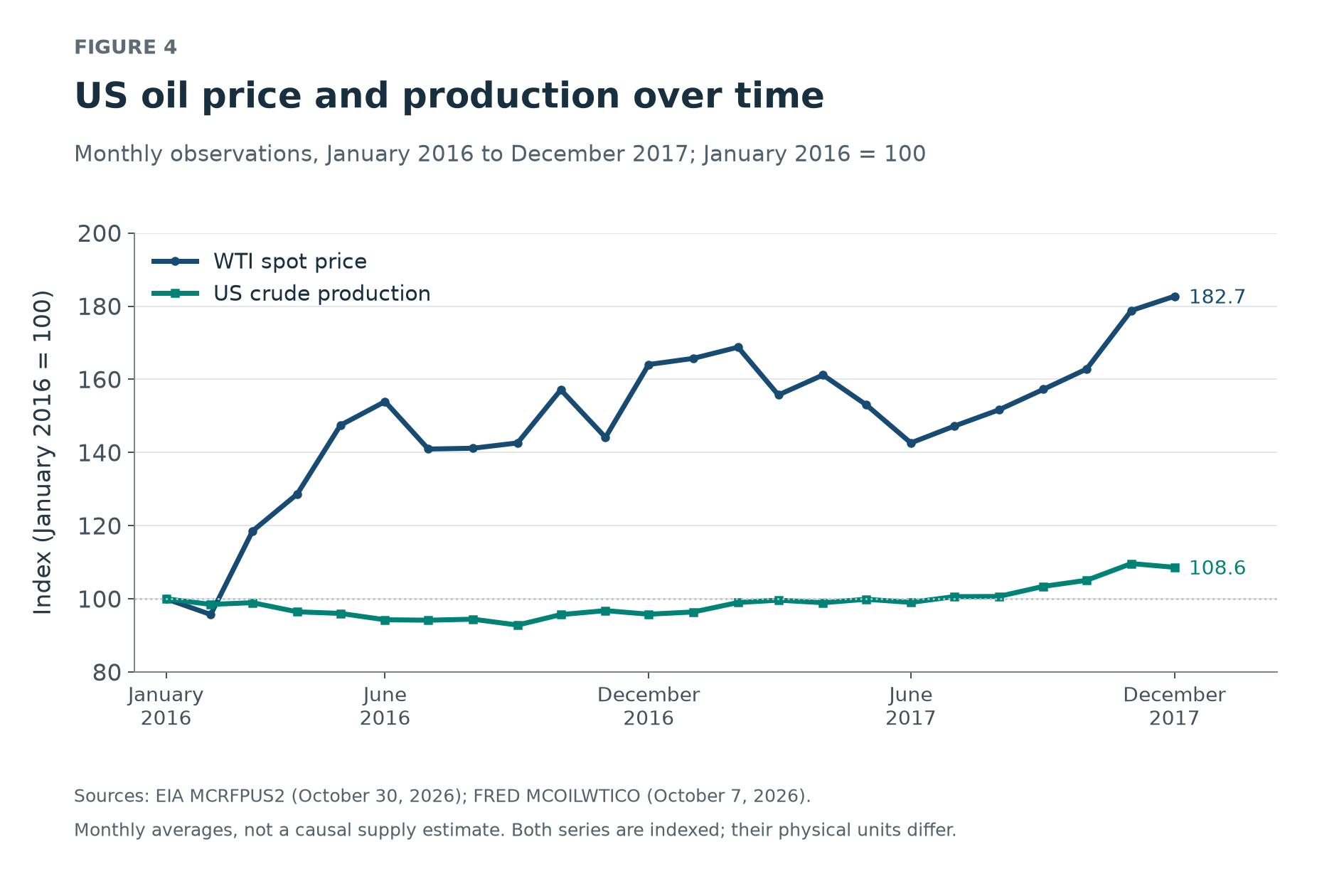
Figure 4. Monthly US crude production and WTI price, January 2016 through December 2017. Each series is indexed to January 2016 = 100 using all 24 reported monthly observations; no missing months are filled. Production is a monthly average daily flow, and WTI is the monthly Cushing spot price in nominal US$ per barrel. Indexing compares proportional changes, not physical units. The series do not isolate a causal price response or estimate supply elasticity. Sources: EIA MCRFPUS2, October 30, 2026 release, and FRED MCOILWTICO, updated October 7, 2026.

The observations show that production did not rise alongside the early price recovery. They cannot determine how much later growth was caused by that recovery, because other production conditions were changing too. Nor does a two-year window establish that every input had fully adjusted. A long-run supply estimate requires an explicit model of the adjustment horizon. [6][8][9]

Entry and investment also need not leave input costs unchanged. If expanding an industry raises wages for scarce skills or the price of suitable land, those costs restrain the eventual increase in supply. A permanently flat long-run market curve requires stronger assumptions than an upward-sloping short-run curve. [6]

Where supply meets demand

Market equilibrium is a price and quantity at which planned purchases equal planned offers. For the constructed bread market, suppose demand is Q_D = 180 - 30P. Supply is Q_S = 30P - 60. Their single intersection is US$4 and 60 loaves per day. Both schedules then specify the same quantity. [1]

At US$3, buyers want 90 loaves while sellers offer 30: the shortage is 60 loaves per day. At US$5, sellers offer 90 while buyers want 30: the surplus is 60. A shortage measures excess planned purchases at the quoted price. A surplus measures excess planned offers. Neither number says how many transactions actually occur.

With flexible prices and the assumed competitive conditions, unfilled orders create pressure for price to rise, while unsold offers create pressure for it to fall. Those adjustments change quantity supplied along the curve unless selling conditions change as well. The intersection describes consistency between plans, without establishing that every household can afford the product. [1]

What a supply curve can establish

Published price and quantity observations are outcomes of buyers' and sellers' decisions together. Connecting them does not recover the supply schedule that held other conditions fixed. Estimation needs identifying assumptions that separate price variation from changes in production conditions. A credible demand shift can reveal movements along supply only if it does not independently shift supply. [10]

Competitive farm commodities provide a stronger setting for this inference when harvest and price data are available and the price variation can be defended. In their 2013 study of corn, rice, soybeans and wheat, Michael J. Roberts and Wolfram Schlenker use past yield shocks to help identify supply: earlier harvest surprises change inventories and futures prices. The inference depends on those shocks providing an appropriate source of price variation. Published quantities alone would not supply that justification. [10]

Inference is weaker when sellers can influence prices through coordinated output decisions. The EIA's oil-market guide describes OPEC setting production targets to influence the market. Such decisions complicate an interpretation of oil price and production movements as adjustments along a competitive supply curve. [11]

At the limiting case of a monopoly, the firm chooses output using marginal revenue, which differs from price because extra sales affect the price it can obtain. Its preferred output depends on the demand it faces as well as its costs. Treating its marginal-cost curve as a competitive supply schedule would omit part of that decision. The competitive diagram is useful when price-taking and the conditions held fixed are defensible for the market being studied. [12]

Sources and further reading

OpenStax, "Principles of Economics", third edition, chapter 3, section 3.1, "Demand, Supply, and Equilibrium in Markets for Goods and Services" (December 14, 2022). Supports supply definitions, schedules, graph axes and equilibrium. The bread schedules and demand equation are original constructed examples.
OpenStax, "Principles of Economics", third edition, chapter 3, section 3.2, "Shifts in Demand and Supply for Goods and Services" (December 14, 2022). Supports the distinction between price movements and supply shifts, including technology, input costs, taxes and subsidies.
Federal Reserve Education, Scott Wolla, "Supply" (undated; accessed November 2, 2026). Supports seller numbers and expected future prices as supply shifters; the transcript credits the Federal Reserve Bank of St. Louis.
OpenStax, "Principles of Economics", third edition, chapter 7, section 7.3, "Costs in the Short Run" (December 14, 2022). Supports marginal cost, fixed and variable costs, and diminishing marginal returns.
OpenStax, "Principles of Economics", third edition, chapter 8, section 8.2, "How Perfectly Competitive Firms Make Output Decisions" (December 14, 2022). Supports price-taking output choice, shutdown and market aggregation. The baker's cost functions are constructed for this article.
OpenStax, "Principles of Economics", third edition, chapter 8, section 8.3, "Entry and Exit Decisions in the Long Run" (December 14, 2022). Supports adjustment horizons, entry and industry input-cost conditions.
OpenStax, "Principles of Economics", third edition, chapter 5, section 5.3, "Elasticity and Pricing" (December 14, 2022). Supports greater opportunities for supply adjustment over longer horizons. The percentage-response definition is given in section 5.1, "Price Elasticity of Demand and Price Elasticity of Supply".
U.S. Energy Information Administration, "U.S. Field Production of Crude Oil", monthly series MCRFPUS2 (October 30, 2026 release). Supplies January 2016 through December 2017 production in thousand barrels per day.
Federal Reserve Bank of St. Louis, FRED, "Crude Oil Prices: West Texas Intermediate (WTI), Cushing, Oklahoma", series MCOILWTICO (updated October 7, 2026). Supplies January 2016 through December 2017 monthly prices; the underlying producer is the U.S. Energy Information Administration.
American Economic Association, Michael J. Roberts and Wolfram Schlenker, "Identifying Supply and Demand Elasticities of Agricultural Commodities: Implications for the US Ethanol Mandate" (October 2013). Supports the use of past yield shocks, inventories and futures prices to identify agricultural supply responses.
U.S. Energy Information Administration, "What Drives Crude Oil Prices: Supply OPEC" (undated; accessed November 2, 2026). Supports the example of coordinated production targets and their implications for oil prices.
OpenStax, "Principles of Economics", third edition, chapter 9, section 9.2, "How a Profit-Maximizing Monopoly Chooses Output and Price" (December 14, 2022). Supports the distinction between monopoly output choice and competitive price-taking supply.