The VLOOKUP Excel Function is used to retrieve data from tables. It comes handy when you have a large dataset and want to retrieve values by entering a value to look for. The “V” stands for “Vertical” lookup.

The value you are looking for must appear in the first column of the table holding your data. It can be an ID, for example.

VLOOKUP also can look up strings.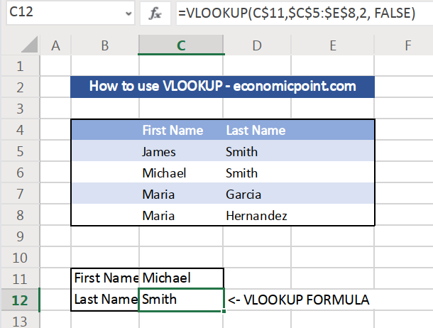

The syntax of the VLOOKUP function is:

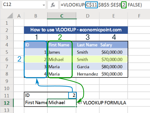
=VLOOKUP(value, table, col_index, [range_lookup])

Where:

- value: the value to look up. In our example, we are looking up an employee id. The table holding our data has the employee id in the first column.

- table: the table that contains our data.

- col_index : to column index from which to retrieve the value. In our example, the first name is in the second column (2), the last name is in the third column (3) and so on.

- range_lookup : this one is optional. It can be TRUE or FALSE. Excel uses TRUE by default. When TRUE, VLOOKUP will allow approximante match, and when FALSE, VLOOKUP will look up an exact match. Usually you want to use FALSE. You can use TRUE if you need the best match.

Warning: Excel default value for range_lookup is FALSE. This means that by default, it can return an incorrect value if the table is not sorted.

This danger posed by Excel defaults is shown in the following clip:

Important Notes:

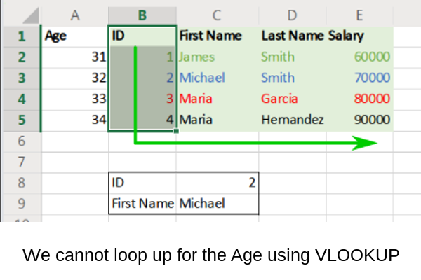
- VLOOKUP only looks for values located to the right of the search column

- VLOOKUP will always find the first match. So for example, if you have duplicate ids for different employees, VLOOKUP will returt the data of the employee located above the second one.

- VLOOKUP is not case-sensitive. For VLOOKUP, Michael is the same as MICHAEL