Example 1: Linear production function

The simplest production function is a linear production function with only one input:

Q = a * L

For example, if a worker can make 10 chairs per day, the production function will be:

Q = 10L

Example 2: Diminishing Returns Production Function

In the linear example, we could keep adding workers to our chair factory and the production function wouldn’t change. If there are 50 workers, the production will be 500 chairs per day. Let’s now take into account the fact that we have fixed capital and diminishing returns.

Q = a * Lb 0<b>1

For example:

Q = 10 * L0.5

Now, the relationship between output and workers can be seeing in the following chart:

Example 3: Production Function with Multiple Inputs

Let’s now take into account the fact that there can be more than one input or factor. Let’s say we can have more workers (L) but we can also increase the number of saws (K).

Q = a * Lb * Kc 0<b<1 0<c<1

For example:

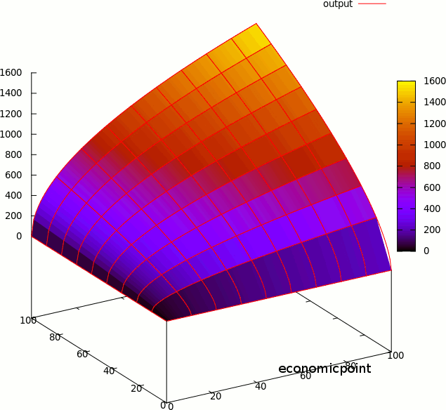
Q = 10 * L0.5 * K0.6

Now, the relationship between output and workers can be seeing in the following plot:

This kind of production function Q = a * Lb * Kc 0<b<1 0<c<1 is called Cobb-Douglas Production Function.

Example 4: Fixed proportions

Let’s assume the only way to produce a chair may be to use one worker and one saw. An additional saw may be useless if we don’t have an additional worker.

This kind of production function is called Fixed Proportion Production Function, and it can be represented using the following formula:

min{L,K}

If we need 2 workers per saw to produce one chair, the formula is:

min{2L,K}

The fixed proportions production function can be represented using the following plot:

Example 5: Perfect Substitutes Production Function

In this example, one factor can be substituted for another and this substitution will have no effect on output.

Let’s say one carpenter can be substituted by one robot, and the output per day will be the same.

The formula for this example is:

Q = a * L + d * R

If we go back to our linear production function example:

Q = 10 * L + 10 * R

Where R stands for the number of robots.

If one robot can make 100 chairs per day, and one carpenter 10:

Q = 10 * L + 100 * R

Example 6: Cobb Douglas Production Functions

This is a particular example of a multiple inputs (Example 3) production function with diminishing returns (Example 2).

The Cobb Douglas production function is widely used in economic models.

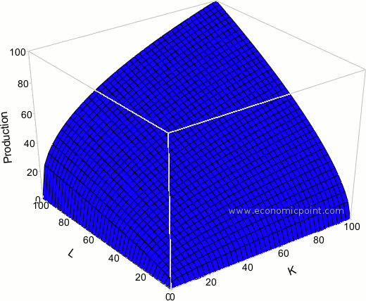
Matehmatically, the Cobb Douglas Production Function can be represented as:

Q(L,K) = A L^β K^α

Where:
- Q is the quantity of products
- L the quantity of labor applied to the production of Q, for example, hours of labor in a month.
- K the hours of capital applied to the production of Q, for example, hours a machine has been working for the production of Q.

Graphically:

This production function has:
- Positive and decreasing marginal product
- Constant output elasticity
- Easy to measure returns to scale (they are obtained from β+α)
- Easy to go from the algebraic form to the linear form, and that makes this function usefull in econometrics models.

Example 8: The Constant Elasticiy of Substution (CES) Production Function

The CES Production function is very used in applied research. It shows a constant change in output, produced due to changes in inputs. Matehmatically, the CES function can be represented as follows:

Q = A[aK^β + (1-a) K^β]^1/β

Where:
Q = Quantity of Output
F = Factor Productivity
a = share parameter
K,L = Quantity of Inputs

The elasticity of substitution is s = 1/(1-β)