Linear Production Function

The linear production function is the simplest form of a production function: it describes a linear relation between the input and the output.

One Input

If the function has only one input, the form can be represented using the following formula:

y = a x

For example, if a worker can produce 10 chairs per day, the production function would be:

Q = 10 L

This function can be represented in the following chart:

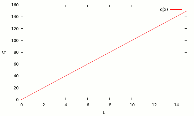
linear production function: one input

The number 10 represents the productivity of labor. If the worker increase it’s productivity, because he took a course on how to produce chairs more quickly, the new production function would be:

Q = 12 L

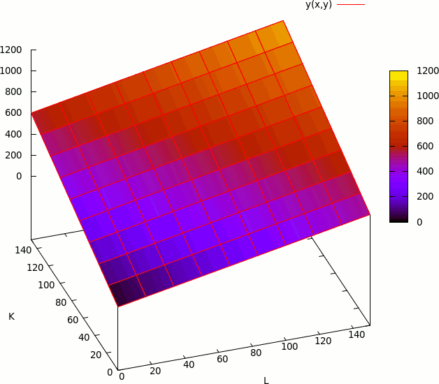
Multiple Inputs

If the function has more than one input:

y = a₁ x₁ + … + a_n x_n

all inputs are perfect substitutes.

linear production function: 2 inputs

Isoquant

Consider the following linear production function:

Q = K + L

This function, has the following isoquant:

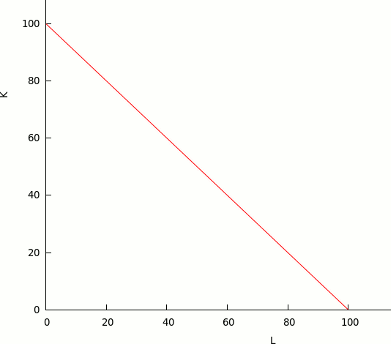
linear production function: isoquant

Please note the lack of a curve in the chart: this show us that the inputs are perfect substitutes

Returns to Scale

Returns to scale measure how much additional output will be obtained when all factors change proportionally.

If the output increases more than proportionally, we say we have increasing returns to scale. If the output increases less than proportionally, we say we have decreasing returns to scale. If the output changes proportionally, we say that the production function has constant returns to scale.

In the case of the linear production function, the returns to scale are constant:

To check how much will output increase when all factors increase proportionally, we multiply all inputs by a constant factor c. Y’ represents the new output level.

Y = aK + bL
Y’ = a (cK) + b (cL)
= c (aK + bL)
= c Y

If all inputs change by a factor of c, output changes by c. The linear production function has constant returns to scale.

Elasticity of substitution

The elasticity of substitution is a measure of how easily can be one factor can be substituted for another. Mathematically, it is defined as the percentage change in factor proportions divided the change in the MRTS (marginal rate of technical substitution), but we will try to understand it in a more intuitive way.

Please take a look to the following isoquant:

isoquant

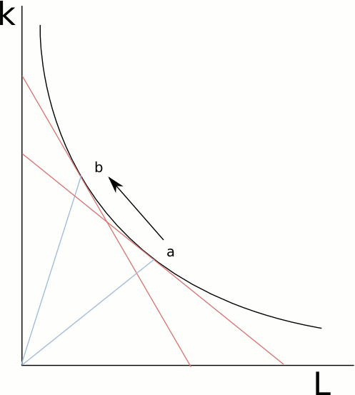
At the point a, the slope of the tangent measures the marginal rate of substitution (MRTS), or how much L can we decrease if we increase K. If we move to the point b, the MRTS increases. This means, that, as we move to the left, we need to add more K for every worker we subtract.

The relation K/L can bee seen by the slope of the straight lines that go from the origin to the points a or b.

The MRTS can be seen by the slope of the tangent to the isoquant.

The elasticity of substitution measures the relation between the change in K/L with the change in the MRTS.

If an isoquant is very curved, the change in the MRTS will be very high in relation to the change in K/L. The elasticity of substitution will be lower: it is very hard to replace one input with another.

Then: if the isoquant is more curved, the elasticity of substitution will be low.

In the case of the linear production function, the MRTS remains constant in the whole range. So the change in the MRTS will be always 0; the denominator is 0.

The change in K/L is not 0. So, we can deduct that the elasticity of substitution, for a linear production function, is ∞.

This conclusion in very straightforward: the inputs are perfect substitutes.